An LLM is trained in stages (Figure 1). Each stage reads less data than the one before, and the data gets cleaner and closer to the conversations the model will have. Pre-training and mid-training produce the base model, which continues any text it is given. Post-training turns it into the model people talk to: first supervised fine-tuning (SFT), then reinforcement learning (RL). AI labs often repeat both in several rounds. An instruct model follows instructions; a reasoning model also writes out its steps before answering.
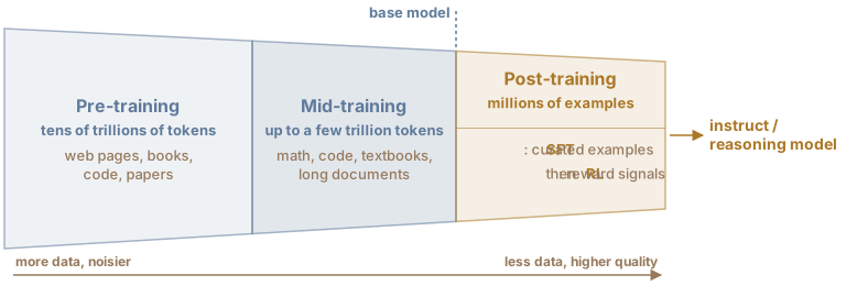
Figure 1:The three training stages: pre-training, mid-training, and post-training (SFT and RL).
Each stage might read the same musical fact in a different form (the texts are illustrative):
| Stage | The same fact, as the model reads it | Learns from |
|---|---|---|
| Pre‑training | Web page: “…top 10 guitar tricks!! #7: G7 to C always sounds like home, try it on your next song…” | Every token |
| Mid‑training | Textbook: “In C major, the dominant seventh G7 resolves to the tonic: the leading tone B rises to C, and the seventh, F, falls to E.” | Every token, in longer, cleaner sequences |
| Post‑training | Conversation. User: “Why does G7 lead to C?” Assistant: “Its B pulls up to C, and its F pulls down to E.” | The answer (SFT) or a reward (RL) |
Pre-training
Pre-training is like reading books without a purpose. There is no task and no human-written label, and the next token is the only target. Much of the work goes into choosing and cleaning the text.
Most of the text comes from web crawls. After the text is extracted from each page, a typical pipeline does three things 12:
Remove duplicates. The web holds many copies of the same text, such as copied articles and text repeated on every page of a site. One sentence appeared more than 60,000 times in a widely used web dataset. Removing copies saves training time, and models trained on deduplicated text reproduce memorized passages about ten times less often 3.
Filter by quality. A small classifier scores each document, for example on its educational value, and low-scoring documents are dropped. Models trained on text filtered this way did much better on knowledge and reasoning tests than models trained on the same amount of text without this filter 1.
Set the data mix. The pipeline sets the share of text from each source, such as web pages, code, and math. Large labs report choosing the mix by training small models on candidate mixes and comparing the results 24.
Before post-training, recent models read tens of trillions of tokens 56. A 300-page book is about 100,000 words, or 130,000 tokens, so these models read the equivalent of well over 100 million books.
Loss spikes
Partway through a large training run, the loss sometimes jumps up suddenly. Such spikes are costly and can make the final model worse 7. Training saves a copy of the weights, a checkpoint, at regular intervals. One large lab reported about 20 spikes in its largest run. Each time, it restarted from a checkpoint saved shortly before the spike. It also skipped the few hundred batches around the spike. A batch is the group of text that the model learns from in one update of its weights. Training on the same batches from an earlier checkpoint caused no spike, so the lab attributed the spikes to particular batches meeting a particular state of the weights, not to bad data alone 8. Another lab found that spikes grew more frequent in larger models. It reduced them by removing passages in which a short sequence of tokens repeats many times. It also changed the way the weights are set at the start, the design of the network, and the training settings 7.
A base model has learned only to continue documents, like the web page and the textbook in the table above. Given “Why does G7 lead to C?”, it may continue with “Why does D7 lead to G?” and more questions like it, as if the request were one item in a list 9. The continuation is illustrative. A few examples in the prompt can still steer a base model (in-context learning).
Mid-training
Toward the end of pre-training, the data mix shifts to the cleanest, most information-rich material, such as textbooks, math, and code 5. This phase is called mid-training 10. Long documents are added around the same time, so that the model learns to use a longer context window 25.
Labs use mid-training to plant skills that post-training later strengthens, such as long step-by-step solutions in math and code 510. The stages overlap: one model family also puts question-and-answer text into its mid-training data 10.
Some music LLMs start from a released base model and continue its pre-training. One study trained such a model further on a few billion tokens of music text and ABC tunes, mixed with general text, then fine-tuned it 11. Audio LLMs (Chapter 2) start from a pre-trained LLM and go through similar stages 1213.
Learning-rate decay and long context
The learning rate sets the size of each update to the weights. Under a schedule that many labs use, it stays constant for most of pre-training and decays toward zero at the end 1415. As it decays, the weights settle and the loss drops sharply 14. Data seen during the decay strongly shapes the final weights, so labs save their best data for this phase, up to a few trillion tokens 141065. This part of mid-training is also called annealing.
In two published reports, the context window grew from thousands of tokens to more than a hundred thousand 26.
Post-training: supervised fine-tuning
Post-training starts with SFT, also called instruction tuning. It teaches the
chat format, instruction following, multi-turn dialogue, and the format for
calling tools (Reasoning, Tool Calling, and Agents). Each
training example is a conversation written out as one token sequence in a chat
template. Figure 2 shows one model family’s template
16; each family has its own. In it, the special tokens
<|im_start|> and <|im_end|>, one vocabulary entry each, open and close each
turn, and the word after <|im_start|> names the speaker. The conversation
often opens with a system prompt: instructions from the app’s developer, such
as “You are a music assistant.”
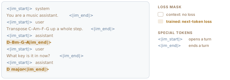
Figure 2:A two-turn conversation in one model family’s chat template 16, as used in SFT. The conversation is illustrative.
The loss is the next-token loss of pre-training, usually applied only to the assistant’s tokens. These include the end-of-turn token, so the model learns to end its turn. The second question, “What key is it in now?”, only makes sense if the model can see the first exchange. The first answer is both a training target and context for the second answer.
Training on answers narrows the base model’s continuations. Raising the probability of an answer after “Why does G7 lead to C?” leaves less probability for other continuations, such as more questions like it.
Early SFT data came largely from people: one early instruction-following model learned from answers written by hired labelers 17. A later study fine-tuned a large base model on only 1,000 carefully chosen examples and obtained a capable chat model. Its authors proposed that most of the knowledge is already in the base model and that SFT mostly teaches format and style 18. Recent public SFT datasets hold about one to two million examples, written by people or generated and then filtered, covering skills such as math, code, and safety 1910.
In one report, a lab ran post-training in rounds and built new SFT examples from its own model. In each round, it sampled many answers per prompt from the previous round’s model and kept the one rated highest by a reward model, a network trained to score answers the way people would. This is called rejection sampling, because the lower-rated samples are thrown away 2.
Open models let anyone download their weights, so you can fine-tune one with SFT on your own examples. Low-rank adaptation (LoRA) freezes the original weights and trains a small set of extra weights added to them, which makes fine-tuning much cheaper 20. Chapter 5, on music education, walks through LoRA fine-tuning of an audio LLM in a code notebook.
Post-training: reinforcement learning
In RL, the model writes its own answers to a prompt, and each answer gets a reward, a number that scores it. Training makes the higher-scoring answers more likely and the lower-scoring ones less likely. Many methods sample a group of answers to the same prompt and compare them.
SFT needs a written answer for every prompt. RL needs only a way to score the model’s own answers, so it also works where full answers are hard to write, such as long step-by-step solutions or descriptions of recordings. Because the model learns from its own answers, it can try ways of answering that nobody wrote down, and training makes the ones that score well more likely. Trying such answers is called exploration. In one lab’s run, RL was applied directly to a base model, with no SFT. Its answers grew steadily longer as it learned to write out more steps before answering 21 (Reasoning).
Start with a request that has one correct answer, the transposition from supervised fine-tuning: “Transpose C–Am–F–G up a whole step.” The model writes three answers, and a program compares each with the reference answer, D–Bm–G–A. A match earns a reward of 1, anything else 0 (the answers are illustrative). Each answer’s advantage is its reward minus the group mean, here 0.33:
| Answer | Mistake | Reward | Advantage |
|---|---|---|---|
| D–Bm–G–A | None | 1 | +0.67 |
| D–B–G–A | B minor became B major | 0 | −0.33 |
| C♯–A♯m–F♯–G♯ | Moved up a half step | 0 | −0.33 |
Training makes answers with a positive advantage more likely and those with a negative advantage less likely 22. The model is never shown the reference answer. It learns only from comparing the scores of its own answers.
If all three answers had scored the same, for example 0 because none was right, every advantage would be zero and the prompt would teach nothing. RL can reward a skill only when some of the model’s own answers already show it. Labs therefore choose prompts that the model gets right only some of the time, and plant skills earlier, in mid-training 22510.
The next example asks an audio LLM to describe a recording: an audio encoder turns the recording into a sequence of vectors, which the LLM reads alongside the prompt’s tokens (Chapter 2).
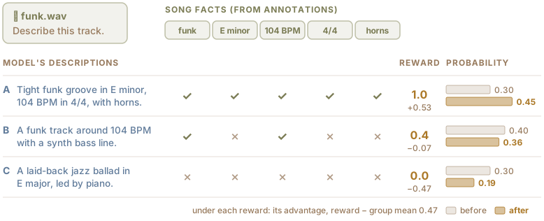
Figure 3:RL on an audio prompt. Each description’s reward is the fraction of annotated facts it matches. Probability is the model’s chance of writing each description, plotted as if the model could write only these three. The number under each reward is its advantage. Track, facts, descriptions, and probabilities are illustrative.
In Figure 3, the model is asked to describe a funk track. Nobody has written a reference description of it to imitate. Its facts are known from annotations: genre, key, tempo, meter, and instruments. Each description’s reward is the fraction of those facts it gets right, a simplified form of a reward used to train one music audio LLM 23. B gets two facts right, a reward of 0.4. That is below the group mean of 0.47, so B becomes slightly less likely.
The update as a loss
Take a prompt and answers with rewards . As a loss, the update is roughly the SFT loss on the model’s own answers. Each answer’s log-probability (the sum over its tokens) is multiplied by its advantage, the reward minus the group mean
Every token of an answer receives that answer’s advantage, so B’s correct “funk” and “104 BPM” are made less likely along with the rest of the description. Both phrases also appear in A, so the total chance of writing them, A’s probability plus B’s, still rises from 0.70 to 0.81.
After SFT, the training signal usually comes from one of two sources:
A check of each answer. In RL with verifiable rewards (RLVR), a program, the verifier, checks each answer against a reference or a rule, such as a known math answer or a test suite for code 1921. Both examples above work this way, and reasoning models learn to write long step-by-step solutions from such rewards.
Choices between two answers. This signal is relative: it says which answer is better, not how good either one is. In RL from human feedback (RLHF), people make the choices, and a reward model learns from those choices to score each answer. A larger gap between two answers’ scores means a higher chance that the higher-scoring one is preferred. This is the Bradley–Terry model of paired comparisons 24. The LLM is then trained with RL to score high on that reward model 2517. Direct Preference Optimization (DPO) learns from the same pairs but trains no separate reward model and samples no new answers, so it is not RL in the strict sense. It makes the preferred answer in each pair more likely relative to the other 26.
Many MIR tasks already have verifiers: a key, a tempo, a list of beat times, or a timed chord sequence can be scored against annotations with the standard metrics in mir_eval 27.
Training on preferences between pairs of answers, by RLHF or DPO, is often called preference tuning. One early model was fine-tuned with SFT and then RLHF. Labelers preferred its answers to those of a model more than 100 times larger that had neither step 17. In music, one study applied RLHF to a text-to-music model that, like an LLM, generates audio tokens one at a time. Its reward model learned from 300,000 pairwise preferences given by the model’s users 28. The preferences can also come from automatic scores or from an LLM acting as a judge (Evaluating LLMs) 19. Another study applied DPO to a model that both understands and generates audio, and picked the preferred output in each pair by how well it matched the prompt and how good it sounded 29.
Labs often combine both sources. They use verifiers where answers can be checked, such as math problems, and preferences for open-ended requests 1921.
Reward hacking
A reward measures only part of an answer’s quality, and a model can learn to exploit the gap. This is called reward hacking 30. The funk reward counts only matches. In Figure 3, C’s wrong key, E major, gets the same ✗ as B, which names no key. A wrong claim costs nothing, so a model trained on this reward may learn to name every common instrument. Practical systems combine several rewards 21 and often penalize the trained model for moving far from the model it started from 17.
- Penedo, G., Kydlíček, H., Ben Allal, L., Lozhkov, A., Mitchell, M., Raffel, C., Von Werra, L., & Wolf, T. (2024). The FineWeb Datasets: Decanting the Web for the Finest Text Data at Scale. Advances in Neural Information Processing Systems, Datasets and Benchmarks Track. https://arxiv.org/abs/2406.17557
- Grattafiori, A., Dubey, A., Jauhri, A., Pandey, A., Kadian, A., Al-Dahle, A., Letman, A., Mathur, A., Schelten, A., Vaughan, A., Yang, A., Fan, A., & others. (2024). The Llama 3 Herd of Models. arXiv Preprint arXiv:2407.21783. https://arxiv.org/abs/2407.21783
- Lee, K., Ippolito, D., Nystrom, A., Zhang, C., Eck, D., Callison-Burch, C., & Carlini, N. (2022). Deduplicating Training Data Makes Language Models Better. Proceedings of the 60th Annual Meeting of the Association for Computational Linguistics (ACL), 8424–8445. 10.18653/v1/2022.acl-long.577
- Gemini Team. (2023). Gemini: A Family of Highly Capable Multimodal Models. arXiv Preprint arXiv:2312.11805.
- Yang, A., Li, A., Yang, B., Zhang, B., Hui, B., Zheng, B., Yu, B., & others. (2025). Qwen3 Technical Report. arXiv Preprint arXiv:2505.09388.
- NVIDIA. (2025). Nemotron 3 Nano: Open, Efficient Mixture-of-Experts Hybrid Mamba-Transformer Model for Agentic Reasoning. arXiv Preprint arXiv:2512.20848. https://arxiv.org/abs/2512.20848
- Team OLMo, Walsh, P., Soldaini, L., Groeneveld, D., Lo, K., & others. (2024). 2 OLMo 2 Furious. arXiv Preprint arXiv:2501.00656. https://arxiv.org/abs/2501.00656
- Chowdhery, A., Narang, S., Devlin, J., Bosma, M., Mishra, G., Roberts, A., Barham, P., Chung, H. W., Sutton, C., Gehrmann, S., & others. (2023). PaLM: Scaling Language Modeling with Pathways. Journal of Machine Learning Research, 24(240), 1–113. https://jmlr.org/papers/v24/22-1144.html
- OpenAI. (2022). Aligning Language Models to Follow Instructions. OpenAI blog. https://openai.com/index/instruction-following/
- Team Olmo. (2025). Olmo 3. arXiv Preprint arXiv:2512.13961. https://arxiv.org/abs/2512.13961
- Yuan, R., Lin, H., Wang, Y., Tian, Z., Wu, S., Shen, T., Zhang, G., Wu, Y., Liu, C., Zhou, Z., & others. (2024). ChatMusician: Understanding and Generating Music Intrinsically with LLM. Findings of the Association for Computational Linguistics: ACL 2024, 6252–6271.
- Tang, C., Yu, W., Sun, G., Chen, X., Tan, T., Li, W., Lu, L., Ma, Z., & Zhang, C. (2024). SALMONN: Towards Generic Hearing Abilities for Large Language Models. The Twelfth International Conference on Learning Representations. https://openreview.net/forum?id=14rn7HpKVk
- Ghosh, S., Goel, A., Kim, J., Kumar, S., Kong, Z., Lee, S., Yang, C.-H. H., Duraiswami, R., Manocha, D., Valle, R., & Catanzaro, B. (2025). Audio Flamingo 3: Advancing Audio Intelligence with Fully Open Large Audio Language Models. Advances in Neural Information Processing Systems. https://papers.neurips.cc/paper_files/paper/2025/hash/3babb6b453cb59d87cb58a1219ef914b-Abstract-Conference.html
- Hu, S., Tu, Y., Han, X., He, C., Cui, G., Long, X., Zheng, Z., Fang, Y., Huang, Y., Zhao, W., & others. (2024). MiniCPM: Unveiling the Potential of Small Language Models with Scalable Training Strategies. arXiv Preprint arXiv:2404.06395. https://arxiv.org/abs/2404.06395
- DeepSeek-AI. (2024). DeepSeek-V3 Technical Report. arXiv Preprint arXiv:2412.19437. https://arxiv.org/abs/2412.19437